Contact

If you have suggestions,
bug reports or
request for improving API/Documentation.

Email: karsar @ ibms.sinica.edu.tw

Importing in Python

Whether in script or in console, there are two main scenarious:

import clustangles as clst
a = clst.Angles()

which means we need to append every class and method with clst
or, in case we don't want to append

from clustangles import *

Inputs and Outputs

Each dataset is represented internally as a 2D numpy matrix, where columns correspond to angles and rows to frames or observations. Clustangles recognizes several file formats such as .csv (comma separated values), output of AMBER traj tool for dihedral angles, as well as dihedral angle outputs from GROMOS and CHARMM. To read a dataset from a .csv file, create an object with an empty dataset, then read data from the file as:

angle = Angles()
angle.read_csv(input-filename, units = “degrees”)

Here default option for units is "degrees" (might be omitted in case of "degrees"), for radians one needs units = "radians". Reading a dataset for an object containing dataset is not allowed, to clean the object run:

angle.clean()

It is possible to convert units from degrees to radians and in opposite direction by using correspondingly angle.to_radians() and angle.to_degrees(). One may create a new object containing a dataset with selected columns (angles) from the old one as:

angle_new = angle.select(1, 4 , 7)

Here, for the sake of convenience, we count columns from one and not from the zero, as it is in Python. This command creates an object containing first, 4th and 7th columns from the old one.
Methods angle.read_amber() and angle.read_charmm() are for obtaining datasets from Amber traj tool and Charmm, Gromos outputs. angle.write() method writes a dataset to .csv file.

An example of angle extraction with MDtraj:

>> import mdtraj as md
>> traj = md.load('ala2.h5')
>> a = Angles()
>> b = Angles()
>> a.add(traj.compute_phi)
>> b.add(traj.compute_psi)
>> a.add_columns(b) # it will contain all psi and phi angles for each frame in trajectory (column as angles, rows as frames)

Circular Statistics

A short description of the meaning of different commands could be obtained by invoking the command help(method_name). As an example, for large_mww_test, the command help(large_mww_test) gives the following:

“Large-sample Mardia-Watson-Wheeler could be applied to several independent samples to establish whether these samples are drawn from a common distribution. It requires sample length to be greater than 10 elements. The null hypothesis is: The distribution is common. ”

Values of descriptors for a particular column may be obtained; for example, the command

mean_direction (angle, 1)

provides a circular mean direction (in units of angle.unit) for the first column of the dataset in the object angle.
For quantities requiring two columns (correlation), the following format should be employed:

circular_correlation (angle_first, 1, angle_second, 3),

where the first column is taken from the dataset in angle_first and the third column from angle_second. Clustangles also provides methods for hypothesis testing of circular statistics results. These include Rayleigh tests for uniformity of circular data with specified and non-specified mean direction, tests for a common mean direction, tests for a common median direction, and tests for a common distribution. Several statistical tests may accept more than two samples, hence the user provides an angles() object containing a dataset, where columns are samples. As an example,

large_mww_test(angle)

provides not only the p-value for the Mardia-Watson-Wheeler test on samples given by the angle object, but some of its interpretation as well. An example output might be:

“The p-value is 0.1202, indicating no significant difference between the distributions from which the samples are drawn.”

PCA

To perform dPCA one runs:

dp = dpca(a)
dp.advice(70)
c = dp.project(2,b,file)

First command creates a dPCA object, second provides some suggestions on how to choose the number of principal components (to describe at least 70% of variance, here), while the last projects dataset in object b onto the first two (2) principal components obtained from the object a. Method returns projection in form of 2D numpy matrix and if file argument is present, writes results to the file.

Unlike dPCA, GeoPCA represents angular data without any transformation as points on a unit hypersphere and determines principle component geodesics. We separate mapping of data points onto a unit hypersphere from computation of the principal component geodesics, since different mappings might be of interest. The default mapping is available as a Angles() method unitsphere():

gp = geopca(angle.unitsphere())

No advice on how to interpret results of GeoPCA is given, as the method implemented currently provides only projection on the first two principal component geodesics. The output of geopca() is an object containing all relevant information about these two principal component geodesics. One may project an angular dataset from object b onto the two principal component geodesics by the command : .project(b.unitsphere()).

To illustrate PCA and GeoPCA on example, we prepared a dataset circles, which is generated via script. The dataset contains three angles with strongly correlating values. For dPCA:

>>> from clustangles import *
>>> a = Angles()
>>> a.read_csv("circles.csv", units="radians")
>>> dp = dpca(a)
>>> c = dp.project(2, a)
Explained 99.1699937271

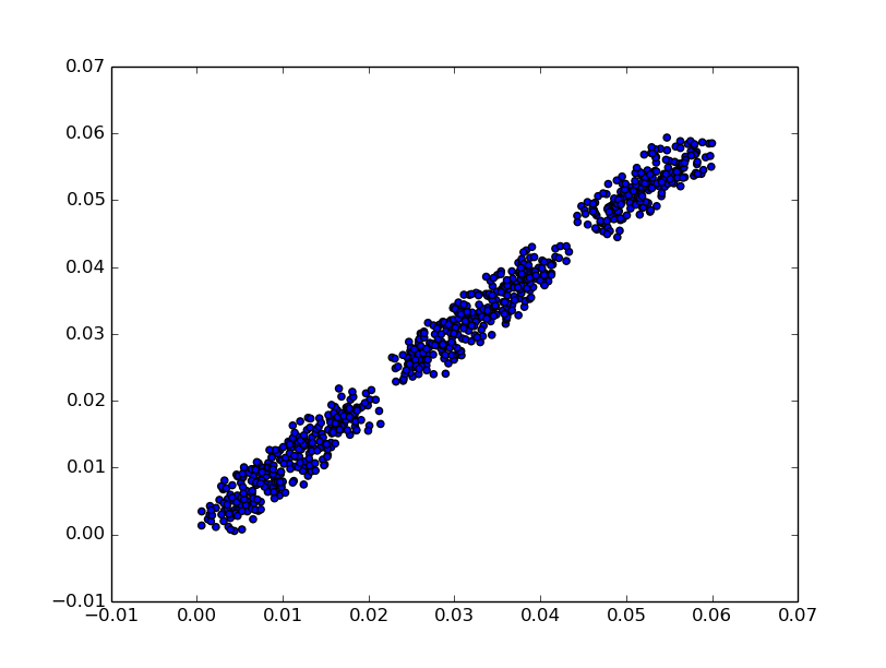
If we plot any pair of angles as (x, y) plot, we obtain a figure similar to one plotted below (first two angles from circles.csv). Matplotlib package is not a part of clustangles, nor is required. User may use other plotting tools. Observe, that the circles.csv dataset is not 2-dimensional! >>> import matplotlib.pyplot as plt
>>> for el in a.dataset:
... plt.scatter(el[0],el[1])
>>>plt.show()

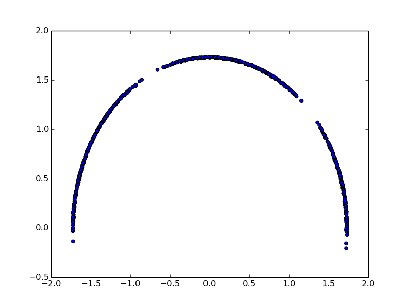
To plot dPCA projection onto the first two principal components:

>>> for el in c:
... plt.scatter(el[0],el[1])
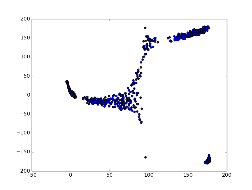
>>>plt.show() For GeoPCA:

>>> geo = geopca(a.unitsphere())
>>> g = geo.project(a.unitsphere())
>>>for el in g.dataset:
... plt.scatter(el[0],el[1])
>>>plt.show() Here, accounting that 180=-180 (output is always in degrees), we divide points into clusters corresponding to those in the first figure [(x,y) plot, or three different steps of generating points for circles.csv].

Clustering

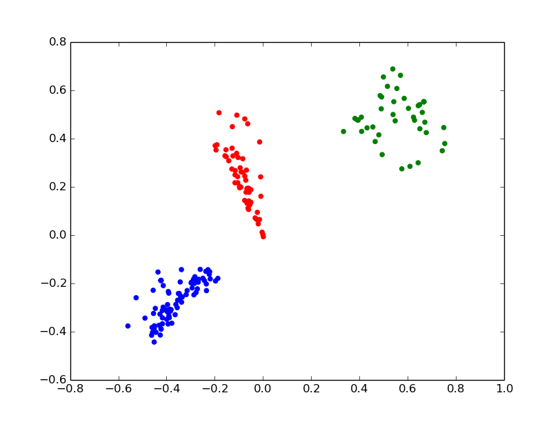
For K-means and hierarchical clustering one first needs to choose whether to use Euclidean distance, or cluster data as point on hypertorus or hypersphere. To illustrate clustering, we prepared a dataset of RNA nucleotides described by their two pseudotorsion angles (rna.csv). It contains three clusters. For every version of K-means we provide a number of clusters we want to get.

>>>b = Angles()
>>>b.read_csv("rna.csv")
>>>k_euc = kmeans(b, 3)
>>>k_torus = kmeans(b, 3, topology="torus")
>>>k_sphere = kmeans(b.unitsphere(), 3, cutoff = 0.5, topology="sphere")

Clusters might be written into the file and plotted as:

>>> k_sphere.write("rna_clusters.csv")
>>> c = Angles()
>>> c.read_csv("rna_clusters.csv")
>>> color=['r', 'g','b']
>>> for el in c.dataset:
... plt.scatter(el[1], el[2], color=color[int(el[0])])
>>>plt.show()

Clustering based on vonMises-Fisher (vmclust) and Watson distributions (wclust) have a similar interface, except only hypersphere topology is allowed. Hierarchical clustering (hclust) takes a threshold distance instead of a number of clusters. It allows Euclidean, hypersphere and hypertorus topologies